Power Approximation for the Test of Study-Level Categorical Moderators in Meta-Regression with Dependent Effect Sizes

Defense of  Bethany Hamilton Bhat

Quantitative Methods Program, The University of Texas at Austin

June 18, 2025

Overview

• Motivating Context for Study

• Review of Power Concepts

• Research Questions

• Methodology

• Results

• Conclusions

• I will begin with the motivation of the study, briefly review some concepts related to power, then move on to my methodology, results, and finally, my conclusions.

Motivating Context for Study

• Dependent effect size estimates in primary studies are prevalent in meta-analyses and models that account for more than one source of dependence are widely used (Pustejovsky and Tipton 2022).
• Inadequate power for a test of moderators can lead to erroneous conclusions.
• Using univariate power analysis methods for a meta-analysis involving dependent effect sizes results in inaccurate power estimates (Vembye et al. 2023)
• Power analysis is available for the test of overall pooled effect size for models that account for dependence (Vembye et al. 2023), but not for the tests of moderators.

While there are univariate power analysis methods for the tests of the overall pooled effect and the tests of moderators, in the context of depend effect sizes which as we know are common in social sciences and educational research, there is only power analysis methods for the test of the overall pooled effect which was proposed by Vembye et al. Extending the work of that study, in this dissertation, I proposed and validated a power approximation formula for the test of equality for study-level categorical moderators when modeling dependent effect sizes.

Power Approximation For Test of Multiple Categories

For the power of cluster-robust Wald test of the equality of multiple categories:

\[ P_{F_{\beta}}(\alpha, \lambda, q) = 1 - F_{F} (c_{\alpha, \nu_n, \nu_d} | \nu_n, \nu_d, \lambda) \]

• \(F_{F}(x|\nu_n, \nu_d, \lambda)\) is the non-central \(F\) distribution function

• \(c_{\alpha,q}\) is the critical value for the central \(F\) distribution with \(\nu_n = C - 1\) and \(\nu_d = \eta_z - (C-1) +1\) degrees of freedom

• \(\lambda\) is the non-centrality parameter: \(\lambda = \sum_{c=1}^C W_{c}(\mu_{c} - \overline{\mu})^2\), where \(\overline{\mu}\) is the weighted grand mean of all the categories.

• I included this slide to highlight that the degrees of freedom used to find power involves the closed form approximation to the HTZ degrees of freedom that are evaluating and that the non-centrality parameter involves the sum of the study-level weights for each category and the overall pooled effect per category. If you woudld like to see the formula for either please me let me know at the end of the talk.

• The non-centrality parameter, NCP or \(\lambda\), is a key parameter in statistical power analysis, and a larger true value for the non-centrality parameter increases statistical power. Since degrees of freedom remain the same under the null and alternative hypotheses, the NCP defines how different the distribution of the alternative hypothesis is from the distribution of the null hypothesis.

Research Questions

Using Monte Carlo Simulation, I aimed to:

1. validate a closed-form approximation of the power for the HTZ test of a categorical study-level moderator based on CHE+RVE.
2. evaluate sampling methods for the sampling variances per study (\(\sigma^2_j\)) and the number of effect sizes per study (\(k_j\)) with the power approximation.
3. evaluate the empirical Type I error rates of the tests of a categorical study-level moderator for the CHE+RVE.

Study Design

In this study, I obtained to types of power estimates.

1. Simulated (true) power
   • Generated through Monte Carlo simulation
     • Design matrix, \(\mathbf{X}\) and vector of meta-regression coefficients, \(\mu_c\)
     • Sampled \(k_j\) and \(\sigma_j^2\) from empirical distribution
     • Standardized Mean Differences Estimates From CHE Model
   • Estimate cluster-robust Wald test of multiple categories using CHE model on simulated dataset and retained p-value: \(r_{\alpha} = \frac{1}{R} \sum_{r = 1}^R I(p_r \lt \alpha)\), where \(\rho_{\alpha} = Pr(p_r \lt \alpha)\).

2. Power Estimates from the Approximation Formula
   • Evaluated three methods for assuming the \(k_j\) and \(\sigma_j^2\) in the approximations:
     • Empirical Distribution
     • Stylized Distribution
       • \(k_j \sim 1 + Poisson(4.56)\) and \(\sigma_j^2 \sim Gamma(1.48, 21.97)\)
     • Balanced

Generating Design Matrix, \(\mathbf{X}\), and Meta-regression Coefficients, \(\mu_c\) for Simulated Data

• To generate \(\mathbf{X}\):
  • use the factors \(C\), \(J_c\), and the balance of the number of studies per category across the moderator

• To generate \(\mu_c\):
  • Given a specified power neighborhood factor in combination with the other specified simulation design factors
    • generated the \(\tilde{w}_{jc}\), the degrees of freedom, the non-centrality parameter of the non-central F-distribution, and the scaling factor to obtain the \(\mu_c\).

• x is clear – mu_c is hard

• if we had use a fixed set that would interact with other design and lead to a restricted power levels. so instead we set we set power neighborhoods – look at conditions that would yield more or less a centerain power level. how ? fix power neighborhood. given . evaluate the approximation across a spectrum of power levels.

• use the arithmetic mean the \(k_j\) and mean \(\sigma^2_j\) of

• using \(\overline{k}_j\), \(\overline{\sigma}^2_j\), \(\tau^2\), \(\omega^2\), and \(\rho\), generate the study-level weights, \(\tilde{w}_{jc}\)

• using \(\tilde{w}_{jc}\) and \(C\), find the degrees of freedom

• using the HTZ formula we derived, \(\eta_z\)

• given \(f_c\), \(\tilde{w}_{jc}\), and \(\lambda\) , find \(\zeta\)

• Using \(\zeta\), \(f_c\), and \(C\), create a vector of coefficients (or \(\mu_c\)).

Correlated-Hierarchical Standardized Mean Differences Estimates

• The \(\boldsymbol{\delta}_j\) had a correlated-and-hierarchical effects structure [CHE; Pustejovsky and Tipton (2022)] and followed the procedures of Pustejovsky and Tipton (2022) and Vembye et al. (2023).
• Sampled \(k_j\) and \(\sigma_j^2\) from Williams et al. (2022).
  • Assumed \(N = \frac{4}{\sigma_j^2}\).
• Assumed effect sizes in each study and across studies are equi-correlated

• Finally, I generated Hedges’ g effect size estimates and the corresponding sampling variance.

Estimation

• For each simulated meta-analytic dataset, I used the CHE+RVE model where I captured the p-value of the Wald’s test of equality of the categories.

• For the value of the assumed \(\rho\), I applied the same sampling correlation value that is used to generate the meta-analytic data.

Simulation Parameters

Parameter	Value
Pattern Type ($f_c$)	2a, 3a, 3b, 3c, 4a, 4b, 4c, 4d
Number of Studies ($J$)	24, 36, 48, 60, 72
Between-study heterogeneity ($\tau$)	0.05, 0.20, 0.40
Within-study heterogeneity ($\omega$)	0.05, 0.20
Sampling correlation ($\rho$)	.2, .5, .8
Power Neighborhood (P)	5%, 20%, 40%, 60%, 80%, 90%
Balance of the $j_c$	balanced $j_c$ vs. imbalanced $j_c$

8,640 conditions

Results - Validating Approximation - RQ1

Results - Validating Approximation - RQ1

• Overestimated power by as much as 20.81 percentage points.

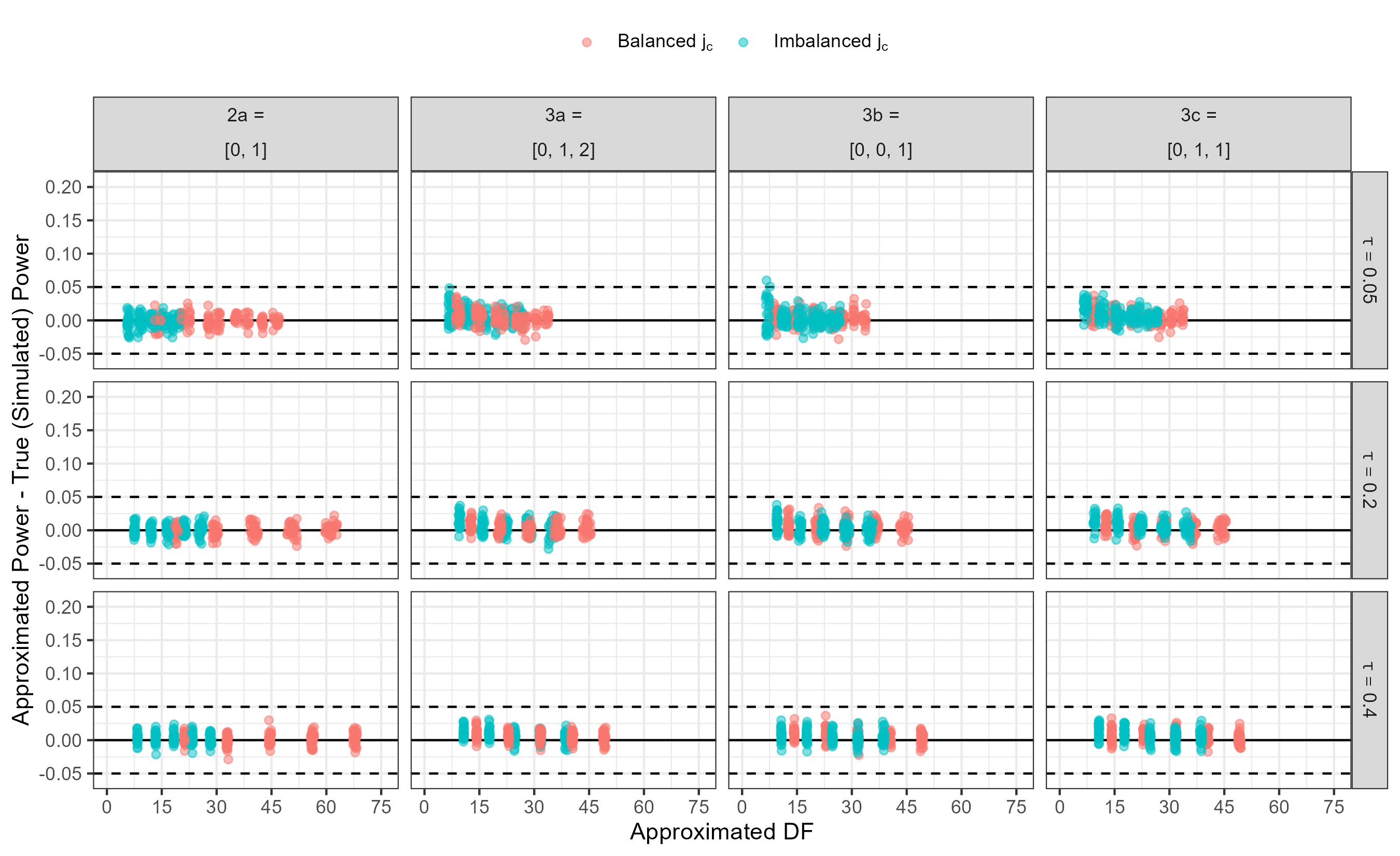
Results - DF Diagnostic - RQ1

• In some conditions, degrees of freedom \(\lt 11.64\) resulted in discrepancies of more than five percentage points.

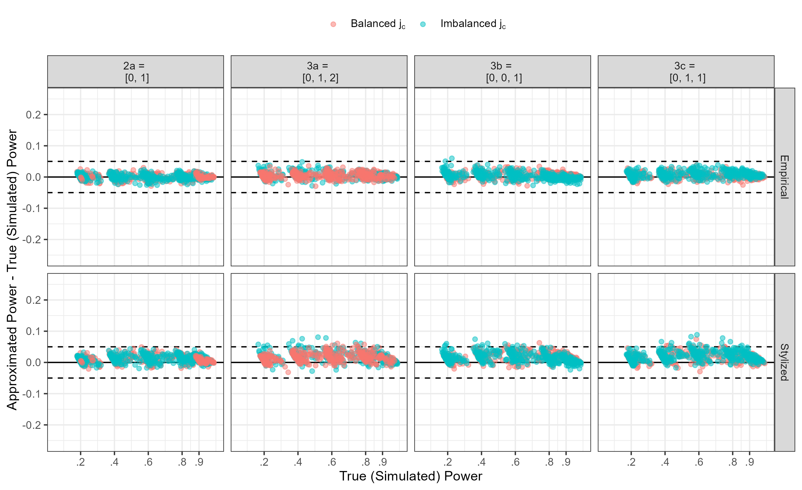
Results - Empirical vs Stylized Sampling Method - RQ2

• Stylized overestimated power by as much as 25.72 percentage points.

• Also, there were some conditions with smaller number of contrasts that stylized sampling method overestimated power by as much as 8.85 percentage points.

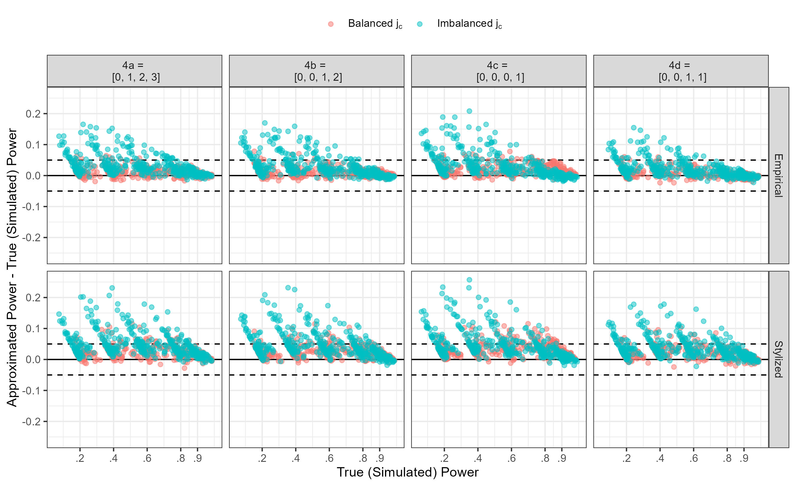
Results - Balanced Sampling Method - RQ2

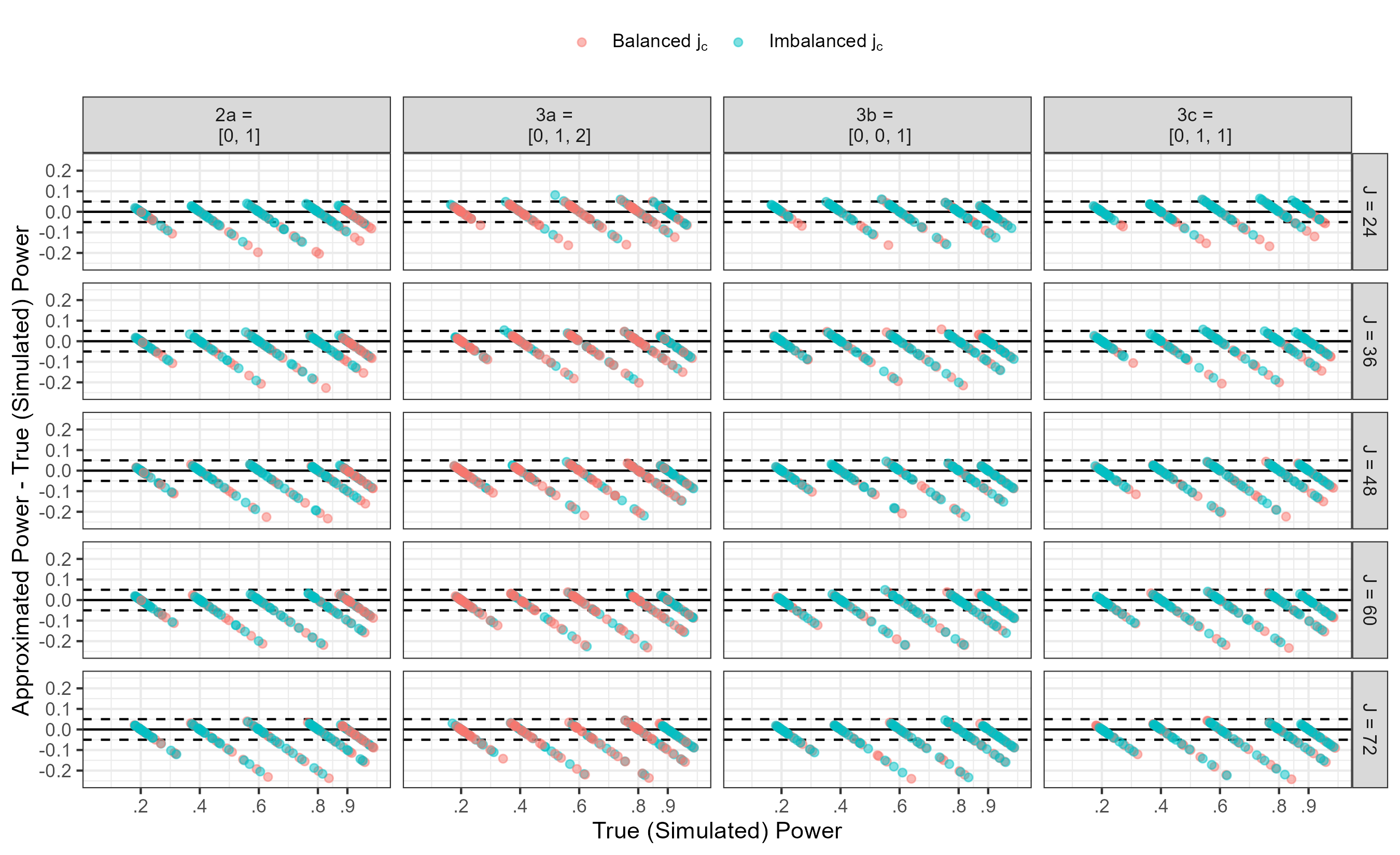
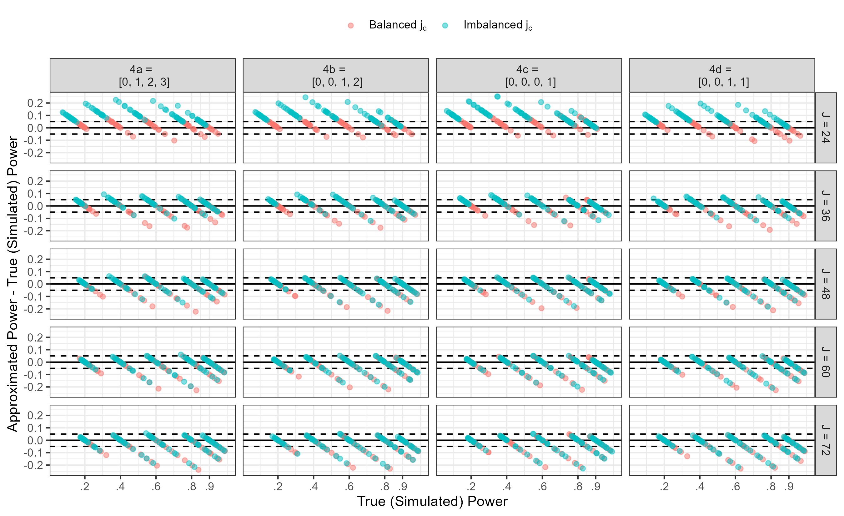
Results - Balanced Sampling Method - RQ2

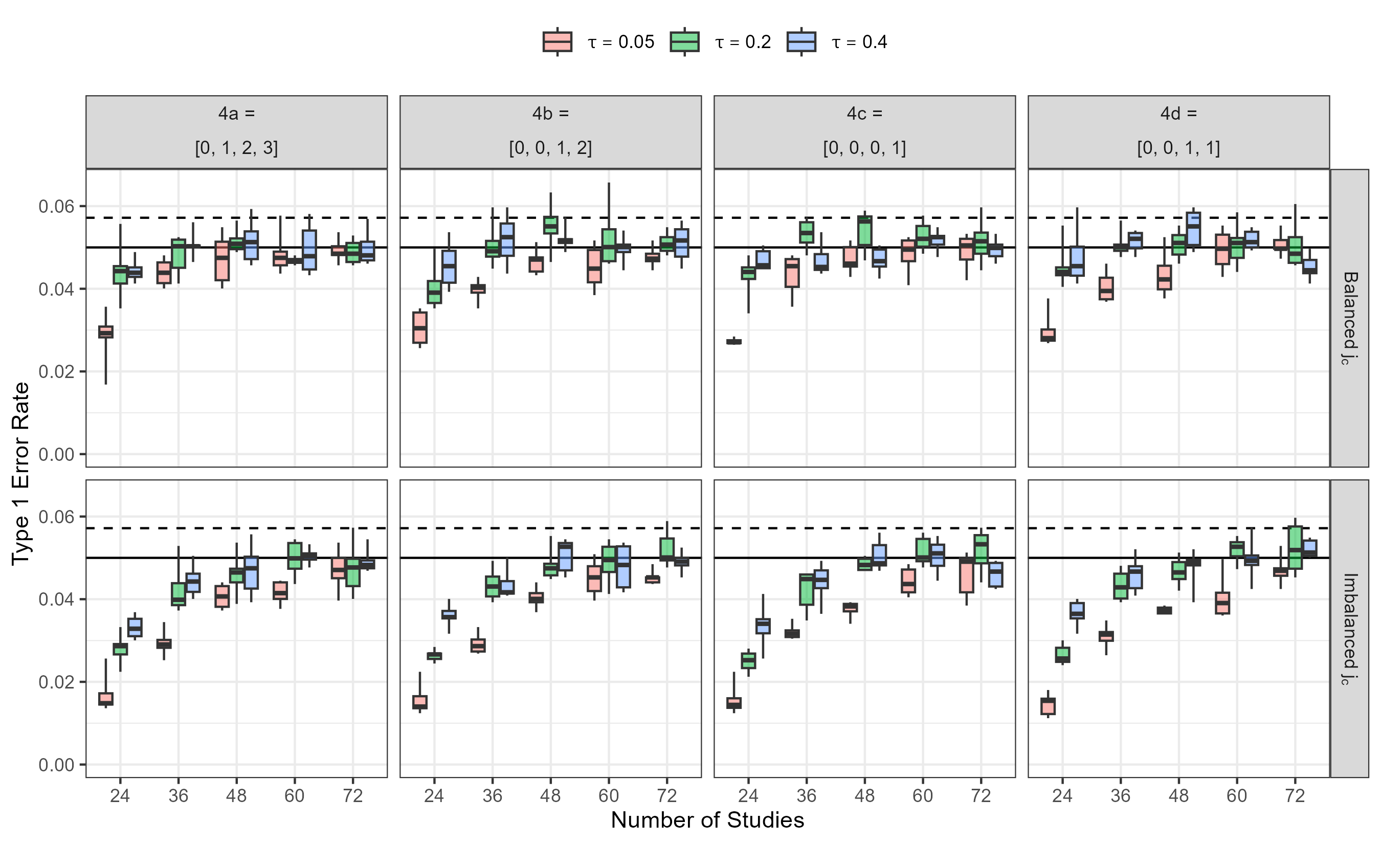
Results - Type I Error Rate - RQ3

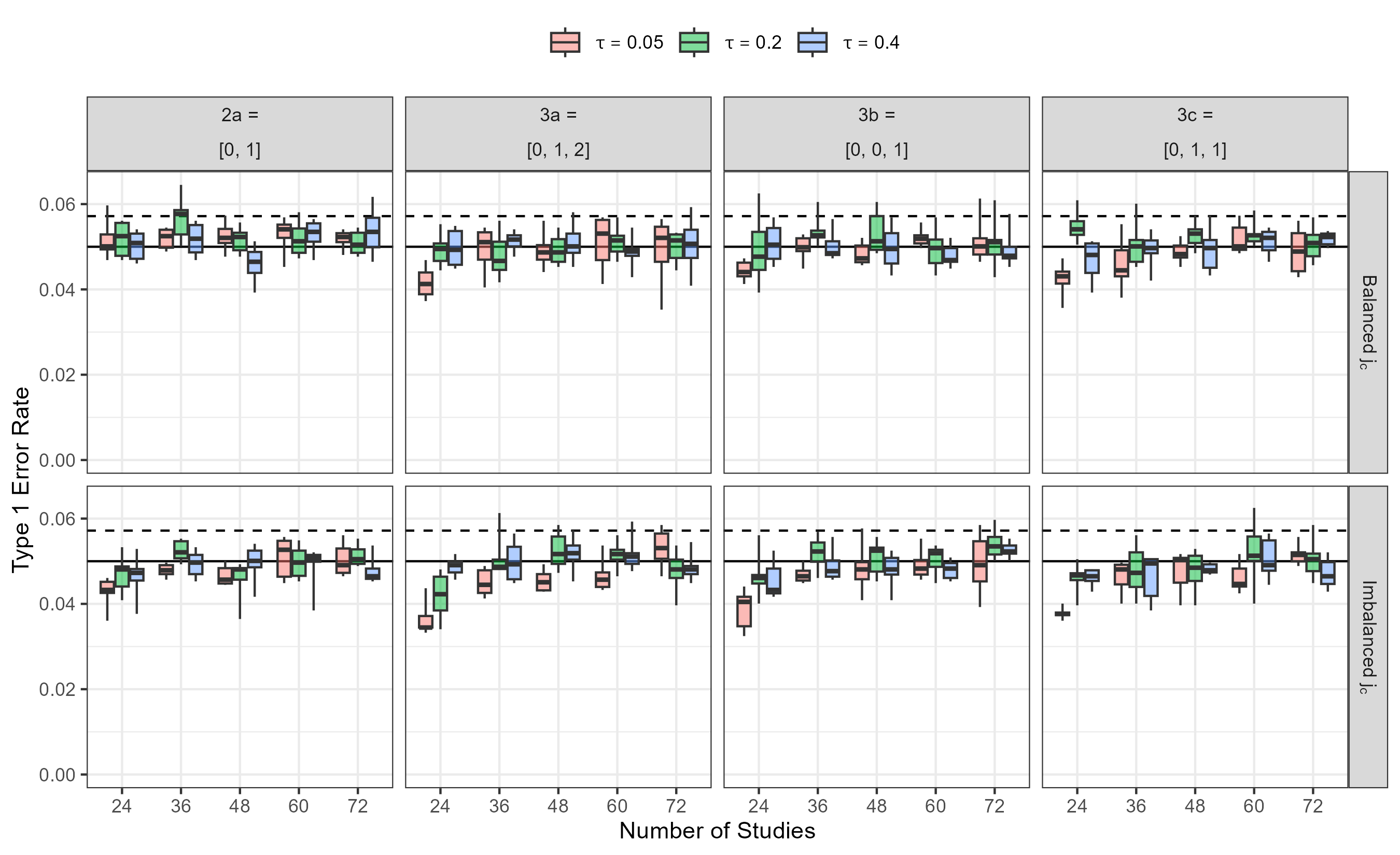
Results - Type I Error Rate - RQ3

Conclusions

I conclude that:

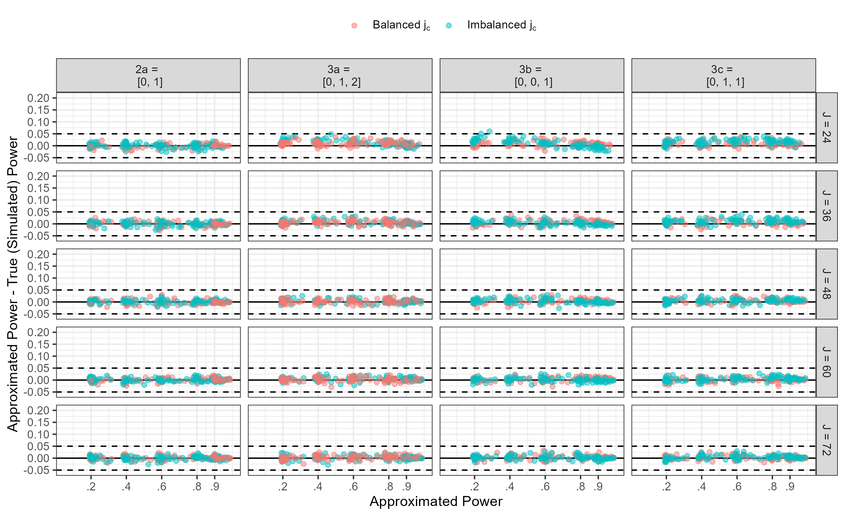
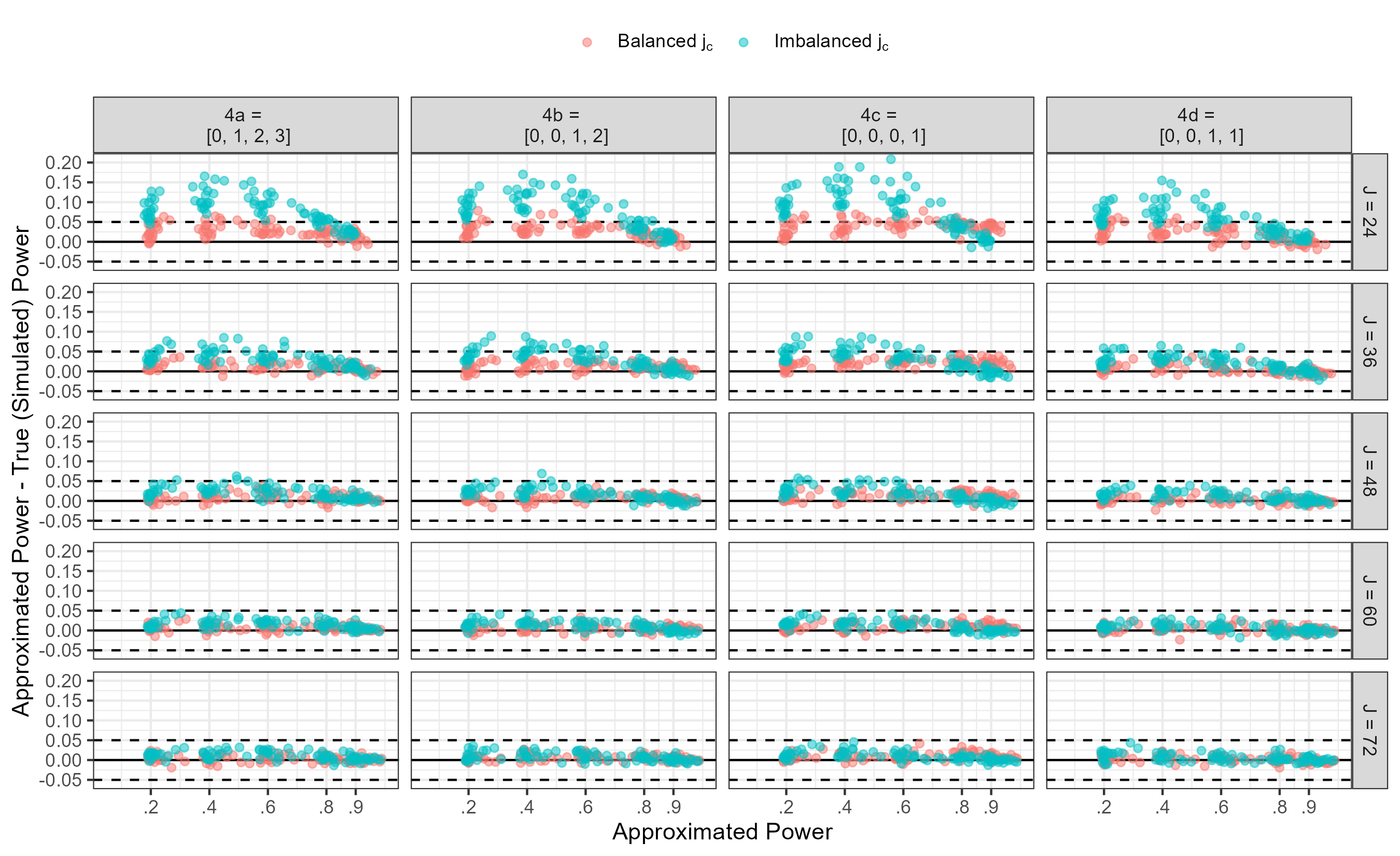
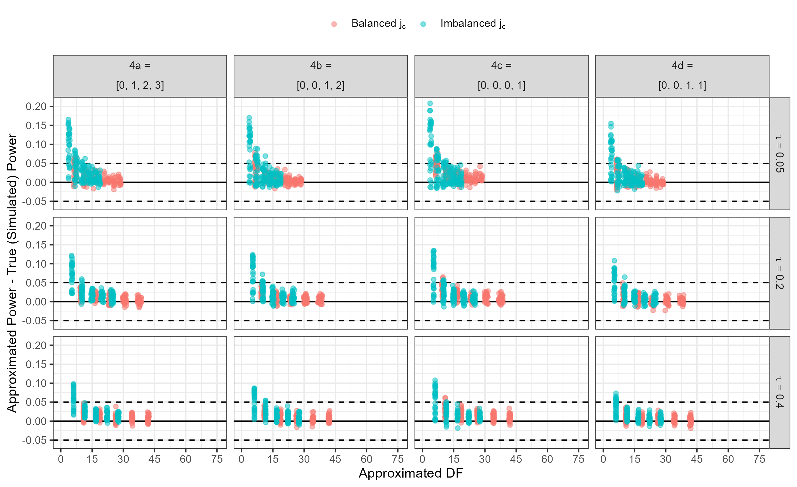
1. The power approximation formula is accurate when there are a small number of contrasts, but it can be inaccurate (overestimates power) in conditions with a larger number of contrasts and small degrees of freedom;

2. It is important to find reliable pilot data for sampling the number of the effect sizes and the sampling variances, as the accuracy of the formula depended on how closely the assumed distributions matched the data generating distributions; and

3. The Type I Error of the robust-Wald Test from a CHE working model was below the nominal error rate, especially in conditions with more contrasts and a small number of total studies.

• 3. replicated findings from Tipton and Pustejov.. 2015 joshi paper

Limitations

• Assumed that the effect sizes in each study and across studies were equally correlated

• Did not examine mis-specification of the between the simulated data and the approximation

• Used one empirical distribution of \(k_j\) and \(\sigma_j^2\) to validate the approximation

• Results will not translate to other effect size types like odds ratio without further assumptions

• Data-generating model was the same as the model used for the approximation

  • Sampling correlation used in the data-generating process is different from the sampling correlation
  • Empirical Distribution used in approximation formula was the same as the data-generating model

Future Directions

• Model-based degrees of freedom (or degrees of freedom for other robust tests) for study-level categorical moderators.

  • Develop power approximations for moderators other than study-level categorical moderators.
  • Validate the approximation under other working models (i.e. \(\rho = 0\) or \(\omega = 0\)).
  • Evaluate if the proposed approximation would work for cluster wild bootstrap test (Joshi et al. 2022).

  • such as the Eigen-decomposition F-test or the Eigen-decomposition and transformation test.

  • Due to the approximation being not performing well with more contrasts and small number of studies, try to…

Acknowledgements

• Committee members:
  • S. Natasha Beretvas (Supervisor)
  • James E. Pustejovsky (co -Supervisor)
  • Teresa D. Pigott
  • Tiffany A. Whittaker
  • Xiao Liu
• I also wanted to acknowledge Megha Joshi and Melissa Rodgers.

References

Joshi, Megha, James E. Pustejovsky, and S. Natasha Beretvas. 2022. “Cluster Wild Bootstrapping to Handle Dependent Effect Sizes in Meta-Analysis with a Small Number of Studies.” Research Synthesis Methods 13 (4): 457–77. https://doi.org/10.1002/jrsm.1554.

Pustejovsky, James E., and Elizabeth Tipton. 2022. “Meta-Analysis with Robust Variance Estimation: Expanding the Range of Working Models.” Prevention Science (New York, Netherlands) 23 (3): 425–38. https://doi.org/10.1007/s11121-021-01246-3.

Vembye, Mikkel Helding, James Eric Pustejovsky, and Therese Deocampo Pigott. 2023. “Power Approximations for Overall Average Effects in Meta-Analysis With Dependent Effect Sizes.” Journal of Educational and Behavioral Statistics 48 (1): 70–102. https://doi.org/10.3102/10769986221127379.

Williams, Ryan, Martyna Citkowicz, David I. Miller, Jim Lindsay, and Kirk Walters. 2022. “Heterogeneity in Mathematics Intervention Effects: Evidence from a Meta-Analysis of 191 Randomized Experiments.” Journal of Research on Educational Effectiveness (Philadelphia) 15 (3): 584–634.

Extra Slides

Results - DF Diagnostic

Results - Empirical vs Stylized Sampling Method

CHE-RVE

• The correlated-and-hierarchical effects (CHE) Model:

\[T_{ij} = \mathbf{x}_{ij}\boldsymbol{\beta} + u_j + v_{ij} + e_{ij}\]

• \(Var(u_j) = \tau^2\), \(Var(v_{ij}) = \omega^2\), \(Var(e_{ij}) = \sigma^2_j\), and \(Cor(e_{hj}, e_{ij}) = \rho\)
• Robust Variance Estimation (RVE):

\[\mathbf{V}^R = \mathbf{M}\left[ \sum_{j=1}^J \mathbf{X}_j' \mathbf{W}_j\mathbf{A}_j\mathbf{e}_j\mathbf{e}_j'\mathbf{A}_j'\mathbf{W}_j\mathbf{X}_j \right]\mathbf{M}\]

• CHE is more comprehensive than other available models that account for dependence since it incorporates both correlated sampling errors and hierarchical dependence, which are both common in meta-analytic datasets. It models the between-study error, within-study error, the sampling error, and assumes a common correlation between sampling errors within a given study.
• working model used to get good estimates of the regression coefficients. robust variance estimation or RVE can be used as an adjustment along side the working model to handle within-study dependence in effect size estimates when estimating the SEs of the \(\beta\) coefficients of meta-regression models.
• where \(\mathbf{e}_j = \mathbf{T}_j - \mathbf{X}_j\bm{\hat{\beta}}\) is the vector of residuals for study \(j\) and \(\mathbf{A}_j\) is a \(k_j \times k_j\) CR2 adjustment matrix
• RVE does not require knowledge of the exact covariance structure between pairs of effect size estimates. Here is the equation for the RVE variance estimator. The variances of the meta-regression coefficients are estimated with sandwich estimators using the cross-product of observed residuals. to estimate the covariance between pairs of effect sizes rather than the known covariances.
• RVE methods can be implemented to maintain close-to-correct Type I error rates even if the CHE model is misspecified. <>

Meta-Regression with Categorical Moderators

• For a no-intercept meta-regression model with a study-level categorical predictor with \(C\) categories:

  \[T_{ij} = \mu_1 b_{j1} +, \cdots, + \mu_{C} b_{jC} + u_j + v_{ij} + e_{ij},\]

• where \(b_{jc}\) is a study-level dummy coded variable and \(\mu_{c}\) is the average effect size for category \(c\) (or the regression coefficient).

• The null hypothesis is \(H_0: \mu_1 = \mu_2 = \cdots = \mu_C\)

• I will use the HTZ-test to test the null hypothesis.

• We derived a closed-form expression for this test statistic and its corresponding degrees of freedom, \(\eta_z\).

Study-level Meta-Regression

• Meta-regression model where the predictors vary at the study level but are constant within a given study.

• Estimation of \(\boldsymbol{\hat{\beta}}\) under CHE: \[\boldsymbol{\hat{\beta}} = \left( \sum_{j=1}^J \tilde{w}_j \mathbf{b}_j' \mathbf{b}_j \right)^{-1} \left( \sum_{j=1}^J\tilde{w}_j \mathbf{b}_j' \overline{T}_j \right)\] where \(\mathbf{b}_j\) is a row vector of study-level categorical moderators, \(x_{ij} = \mathbf{b}_j\) and \(\mathbf{X}_j = \mathbf{1}_j \mathbf{b}_j\), \(\tilde{w}_j = \mathbf{1}_j' \boldsymbol{W}_j \mathbf{1}_j\), \(\mathbf{1}_j\) is a \(k_j \times 1\) column vector, and $

• Study-Level CHE Weights: \[\tilde{w}_j = \frac{k_j}{k_j\hat{\tau}^2 + k_j\rho\sigma_j^2 +\hat{\omega}^2 + (1- \rho)\sigma_j^2}\]

\(\eta_z\)

HTZ test degrees of freedom for multiple categories:

\[\eta_z = \frac{C(C+1)}{2\sum_{c=1}^C \frac{1}{\nu_c}\left(1 - \frac{1}{\psi_c\mathbf{W} } \right)^2}\] where \(\psi_c\) is the expected value of \(V^R\) for each category, \(\frac{1}{W_c}\), and \(\nu_c\) is the degrees of freedom for each category: \[ \nu_c = \left[ \sum_{j = 1} ^{Jc} \frac{w^2_{jc}}{ (W_c - w_{jc}) ^2} - \frac{2}{W} \sum_{j = 1} ^{Jc} \frac{w_{jc}^3}{(W_c - w_{jc})^2} + \frac{1}{W_c^2} \left(\sum_{j = 1} ^{Jc} \frac{w_{jc}^2}{W-w_{jc}} \right)^2 \right]^{-1}\]

Generating Design Matrix, \(\mathbf{X}\), and Meta-regression Coefficients, \(\mu_c\) for Simulated Data

• To generate \(\mathbf{X}\):
  • use the factors \(C\), \(J_c\), and the balance of the number of studies per category across the moderator
• To generate \(\mu_c\):
  • use the arithmetic means for the \(k_j\) and \(\sigma^2_j\) obtained from Williams et al. (2022)
  • using \(\overline{k}_j\), \(\overline{\sigma}^2_j\), \(\tau^2\), \(\omega^2\), and \(\rho\), generate the study-level weights, \(\tilde{w}_{jc}\)
  • using \(\tilde{w}_{jc}\) and \(C\), find the degrees of freedom
  • given the specified power neighborhood level, \(\tilde{w}_{jc}\), the degrees of freedom, \(C\), and an \(\alpha\)-level of \(.05\), generate the non-centrality parameter of the non-central F-distribution, \(\lambda\), using numerical methods.
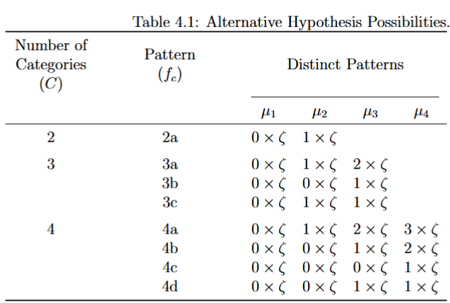
  • given \(f_c\), \(\tilde{w}_{jc}\), and \(\lambda\) , find \(\zeta\)
  • Using \(\zeta\), \(f_c\), and \(C\), create a vector of coefficients (or \(\mu_c\)).

Patterns